- tags
- Cellular automata
- resources
- Wolfram Mathworld, Wikipedia
ECA are one of the simplest form of 1D cellular automata possible. The grid is a 1-dimensional array of cells in state 0 or 1 (dead or alive). The size of the neighborhood being used for the update is 3 (one cell to the left, the main cell and one cell to the right).
Each of those \(2^3\) neighborhoods of size 3 can be mapped to either state 1 or 0. There are \(2^{2^3} = 2^8 = 256\) possible mappings and therefore 256 possible ECA rules.
From this very simple definition, rules with various unexpected behavior emerge. Wolfram constructed a classification of those behavior, known as Wolfram’s classification (Wolfram 2002).
Computational hierarchy
ECA can be listed exhaustively and they represent all the available ways of computing within some strict constraints. One may wonder if some are better than others at computing some things? Or faster, more efficient? Some automata seem to be unable to compute anything like rule 30 whereas some are Turing complete: rule 110 (Cook 2004).
(Hudcová, Mikolov 2021) explores some ways such a hierarchy could be constructed.
Simple implementation
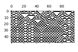
In Python, taking advantage of Numpy’s array manipulation. This implementation is much faster than looping through elements of the grid to update them, but uses slightly more memory. The algorithm is simply based on the standard ECA update.
import numpy as np
import matplotlib
import matplotlib.pyplot as plt
fig, ax = plt.subplots(figsize=(3,2))

N = 100 # Number of cells in the cellular automaton
T = 50 # Number of steps to run for
rule = 54 # Rule code
rule_list = bin(rule)[2:]
# Zero padding of the rule
rule_list = [0] * (8 - len(rule_list)) + [int(i) for i in rule_list]
# Convert to array and reverse the list
rule_array = np.array(rule_list[::-1])

# Initial state
init = np.random.randint(2, size=N)

# We initialize a grid with T rows and N columns
grid = np.zeros((T, N), dtype=np.int)
grid[0, :] = init

for i in range(1, T):
    next_step = rule_array[np.roll(grid[i-1, :], -1) +
                           2 * grid[i-1, :] +
                           4 * np.roll(grid[i-1, :], 1)]
    grid[i, :] = next_step

# Plotting the results
ax.matshow(grid, cmap='Greys')
fig.tight_layout()
fig.savefig('img/plots/ca_rule54.png')
Results:
Bibliography
- Stephen Wolfram. . A New Kind of Science. Wolfram Media. https://www.wolframscience.com/nks/.
- Matthew Cook. . "Universality in Elementary Cellular Automata". Complex Systems, 40.
- Barbora Hudcová, Tomas Mikolov. . "Computational Hierarchy of Elementary Cellular Automata". In . MIT Press. DOI.
Loading comments...